Step-by-Step Guide: Designing Dynamic Table Headers in Excel Spreadsheets

Microsoft Excel becomes a powerhouse once you get into its expansive list of sorting options. Here we’ll cover its most straightforward option for sorting, a simple option that enables us to reorder data in specific columns.

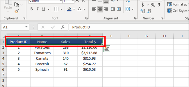
In your spreadsheet, highlight the row with the headings you want to sort. If you don’t want to sort all of the data, you can also just select those cells you need by highlighting them, or by holding Ctrl and clicking to choose multiple unconnected cells.

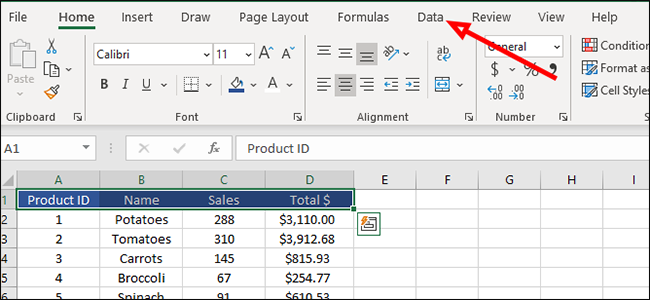
From the top of the page, click “Data” to switch tabs.

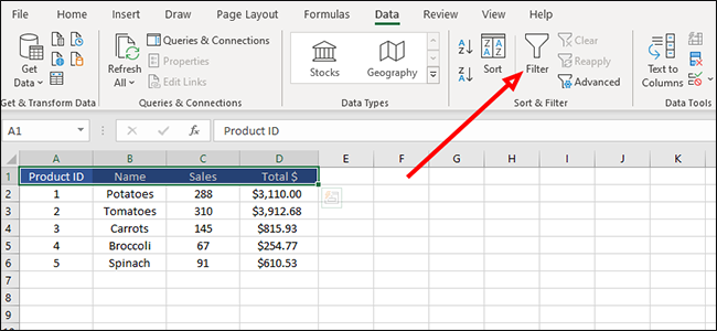
Locate “Sort & Filter,” then click the “Filter” icon. This will add a small down arrow to the right of each heading.

Click the arrow next to “Total $” and sort by largest to smallest or smallest to largest by clicking the appropriate option in the dropdown. This option works for any number, so we can also use it for the “Sales” and “Product ID” sections.

Words, on the other hand, are sorted differently. We can sort these alphabetically (from A to Z or Z to A) by clicking the arrow next to “Name” and then choosing the appropriate option from the dropdown.

Sorting also works by date. If we add an additional column (following the steps above to make it sortable) with dates, we can sort inventory by what’s fresh and what is nearing its sell-by date. We do this by clicking the arrow next to “Received” and choosing to sort from oldest to newest or newest to oldest.

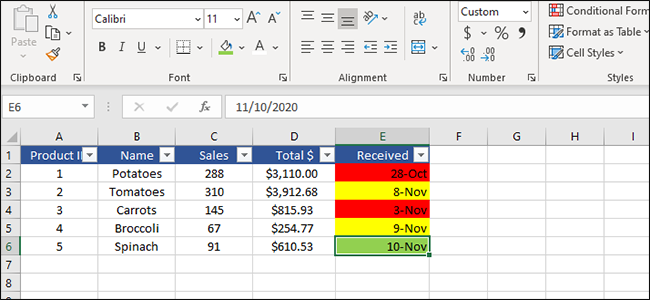
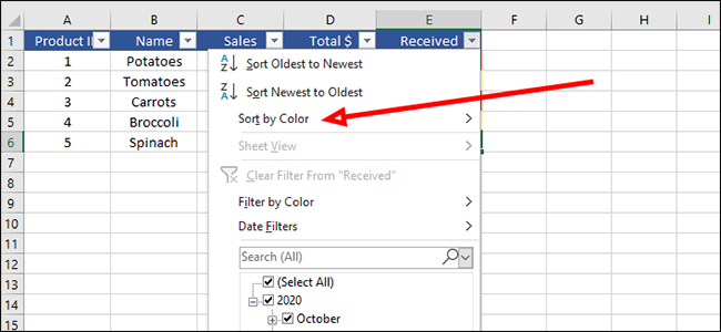
Following up on this example, let’s say we want to label items that need to be sold quickly. We can label the dates with a simple green, yellow, and red system to show items that will be good for a few days, those that are nearing their sell-by date, and those that have to go immediately. We can then sort these by color, to put the red items at the top of the list.

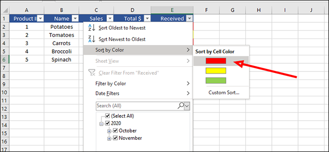
To sort this, click the arrow next to “Received” and choose “Sort by Color.”

Click the cell color you want atop your list. In our case, we’ll select red so we can see the items about to spoil. This is easy to visualize in our example, as we only have five items. But imagine if this was a list with 500 entries instead. Sorting by color becomes much more useful then.

Now you can make any type of Excel spreadsheet data sortable in just a few clicks.

Also read: