Expert Tips and Tricks: Leveraging the Power of Text Splitting in Excel

Quick Links

• Text to Columns with Delimited Text
• Text to Columns with Fixed Width Text
• Converting US Dates to European Format
• Converting International Number Formats

Excel’s Text to Columns feature splits text in a cell into multiple columns. This simple task can save a user the heartache of manually separating the text in a cell into several columns.

We’ll start with a simple example of splitting two samples of data into separate columns. Then, we’ll explore two other uses for this feature that most Excel users are not aware of.

Text to Columns with Delimited Text

For the first example, we will use Text to Columns with delimited data. This is the more common scenario for splitting text, so we will start with this.

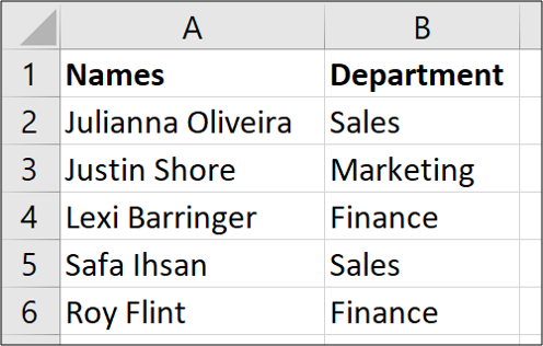
In the sample data below we have a list of names in a column. We would like to separate the first and last name into different columns .

In this example, we would like the first name to remain in column A for the last name to move to column B. We already have some information in column B (the Department). So we need to insert a column first and give it a header.

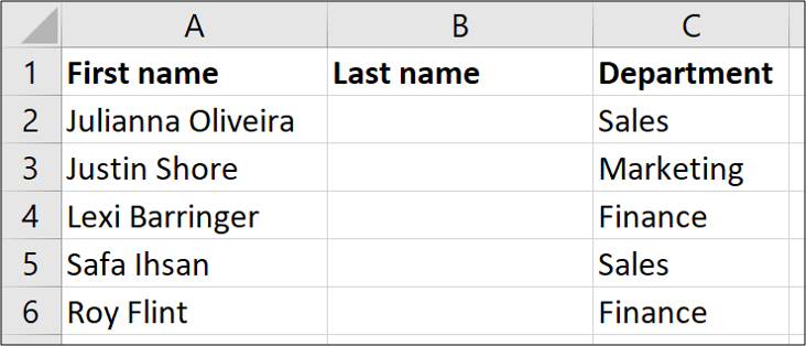
Next, select the range of cells containing the names and then click Data > Text to Columns

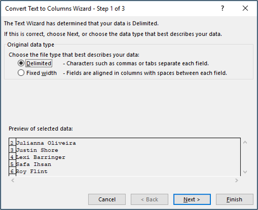
This opens a wizard in which you’ll perform three steps. Step one is to specify how the content is separated. Delimited means the different pieces of text you want to pull apart are separated by a special character such as space, comma, or slash. That’s the one we’re going to choose here. (We’ll talk about the fixed width option in the next section.)

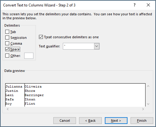
In the second step, specify the delimiter character. In our simple example data, the first and last names are delimited by a space. So, we’re going to remove the check from the “Tab” and add a check to the “Space” option.

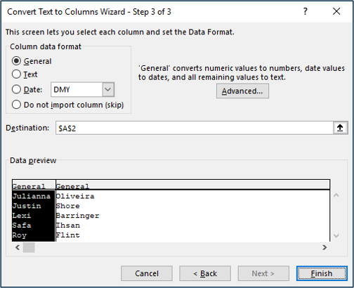
In the final step, we can format the content. For our example, we do not need to apply any formatting, but you could do things like specify whether the data is in the text or date format, and even set it up so that one format converts to another during the process.

We will also leave the destination as $A$2 so that it splits the name from its current position, and moves the last name into column B.

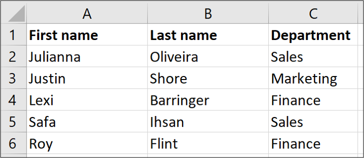
When we click “Finish” on the wizard, Excel separates the first and last names and we now have our new, fully populated Column B.

Text to Columns with Fixed Width Text

In this example, we will split text that has a fixed width. In the data below, we have an invoice code that always begins with two letters followed by a variable number of numeric digits. The two-letter code represents the client and the numeric value after it represents the invoice number. We want to separate the first two characters of the invoice code from the numbers that succeed it and deposit those values into the Client and Invoice No columns we’ve set up (columns B and C). We also want to keep the full invoice code intact in Column A.

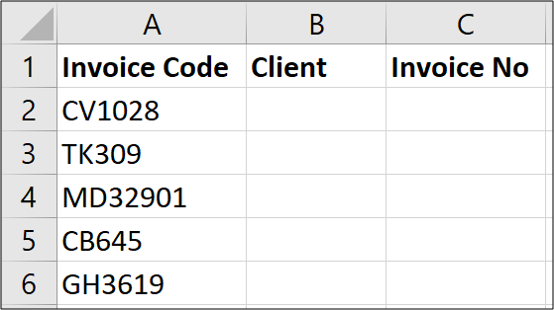
Because the invoice code is always two characters, it has a fixed width.

Start by selecting the range of cells containing the text you want to split and then clicking Data > Text to Columns.

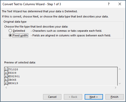
On the first page of the wizard, select the “Fixed Width” option and then click “Next.”

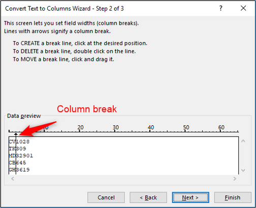
On the next page, we need to specify the position(s) in the column to split the content. We can do this by clicking in the preview area provided.

Note: Text to Columns sometimes provides a suggested break(s). This can save you some time, but keep an eye on it. The suggestions are not always correct.

In the “Data Preview” area, click where you want to insert the break and then click “Next.”

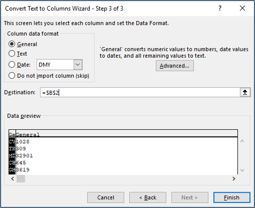
In the final step, type cell B2 (=$B$2) in the Destination box and then click “Finish.”

The invoice numbers are successfully separated into columns B and C. The original data remains in column A.

So, we’ve now looked at splitting content using delimiters and fixed widths. We’ve also looked at splitting text in place and splitting it to different places on a worksheet. Now let’s look at two extra special uses of Text to Columns.

Converting US Dates to European Format

One fantastic use of Text to Columns is to convert date formats. For example, converting a US date format to European or vice versa.

I live in the UK so when I import data into an Excel spreadsheet, sometimes they are stored as text. This is because the source data is from the US and the date formats do not match the regional settings configured in my installation of Excel.

So, its Text to Columns to the rescue to get these converted. Below are some dates in US format that my copy of Excel has not understood.

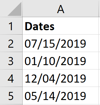
First, we’re going to select the range of cells containing the dates to convert and then click Data > Text to Columns.

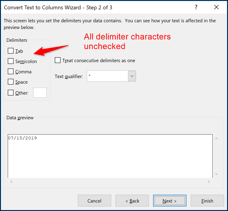
On the first page of the wizard, we’ll leave it as delimited and on the second step, we’ll remove all the delimiter options because we don’t actually want split any content.

On the final page, select the Date option and use the list to specify the date format of the data you have received. In this example, I will select MDY—the format typically used in the US.

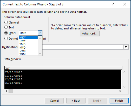
After clicking “Finish,” the dates are successfully converted and are ready for further analysis.

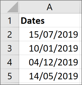
Converting International Number Formats

In addition to being a tool for converting different date formats, Text to Columns can also convert international number formats.

Here in the UK, a decimal point is used in number formats. So for example, the number 1,064.34 is a little more than one thousand.

But in many countries, a decimal comma is used instead. So that number would be misinterpreted by Excel and stored as text. They would present the number as 1.064,34.

Thankfully when working with international number formats in Excel, our good friend Text to Columns can assist us with converting these values.

In the example below, I have a list of numbers formatted with a decimal comma. So my regional settings in Excel have not recognized them.

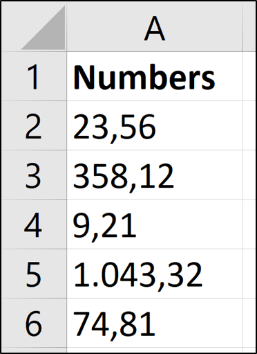
This process is almost identical to the one we used for converting dates. Select the range of values, head to Data > Text to Columns, select the delimited option, and remove all the delimiter characters. On the final step of the wizard, this time we’re going to choose the “General” option and then click the “Advanced” button.

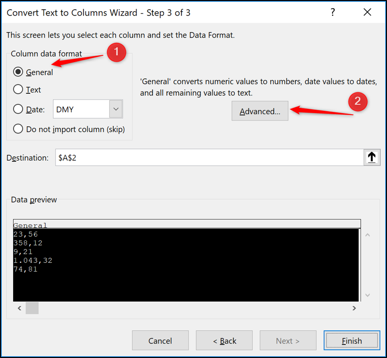
In the settings window that opens, enter the character you want to use in the Thousand separator and Decimal separator boxes provided. Click “OK” and then click “Finish” when you get back to the wizard.

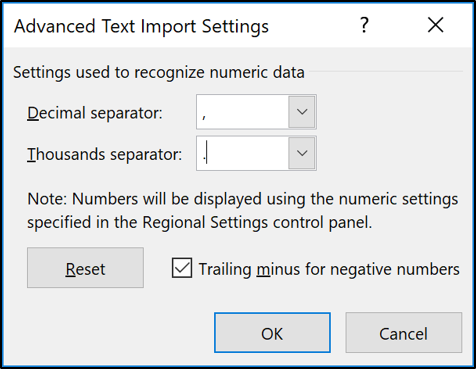
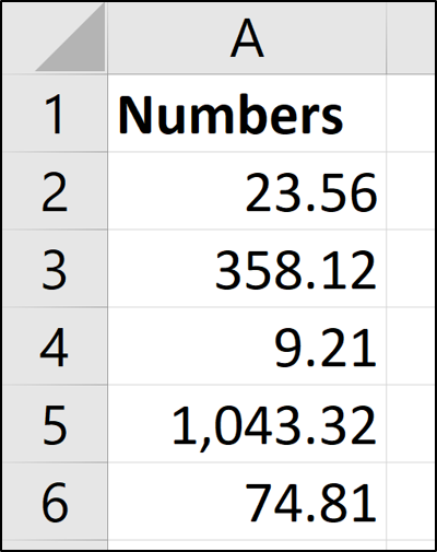
The values are converted and now recognized as numbers for further calculation and analysis.

Text to Columns is more powerful than people realize. Its classic use to separate content into different columns is incredibly useful. Especially when working with data we receive from others. The lesser-known abilities to convert date and international number formats are magic.